59 Background
59.1 Overview of Genarative Model
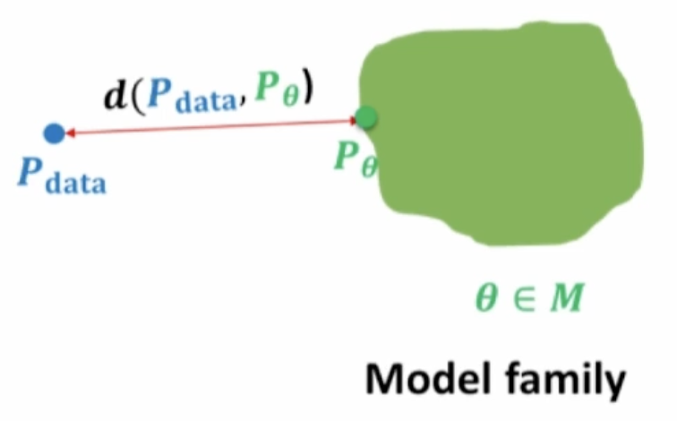
The main task in generative models is to build a model that approximates a probability \(P_{\theta}\) from a set of data points sampled from the true distribution \(P_{data}\) (\(P_{\theta}\) should be as close as possible to \(P_{data}\) according to some distance measure)
We want to learn a probability distribution \(p(x)\) over data \(x\) (e.g., Images, Text, Protein Sequence). These distributions could be used for
Generation: Sample \(x_{new} \sim p(x)\)
Density Estimation: \(p(x)\) should be high if \(x\) is part of the data (anomaly detection)
Unsupervised Representation Learning: Feature extraction
59.2 The Curse of Dimensionality
Representing \(p(x)\) is difficult for high-dimensional data (such as images and text). This is easier, however, for simpler data. For example, a Categorical Distribution (n-sided cube) can be parameterized using \(n-1\) parameters (one for the probability of each outcome and the last is calculated from the first \(n-1\)).
This isn’t the case for high-dimensional data. A single pixel in an image, for example, needs \(256*256*256 - 1\) parameters. For an image, the number of required parameters grows exponentially with the number of pixels.
59.2.1 Independence Assumption
One way to simplify the structure is to assume independence
\[ p(x_1, ..., x_n) = p(x_1)p(x_2)...p(x_n) \]
This would require only \(n\) parameters (because \(p(x_i)\) needs only one parameter) to model the \(2^n\) images.
The problem is that this assumption is way too strong. For example, if you are generating images, you are not allowed to see any other pixel value when extracting the value of a pixel.
59.2.2 Conditional Independence Assumptions
Using the chain rule, you can simplify a multivariate distribution to
\[ p(x_1, ...., x_n) = p(x_1)p(x_2|x_1)p(x_3|x_1,x_2)...p(x_n|x_1,...,x_{n-1}) \]1
The number of parameters, however, is still exponential
\[ 1 + 2 + ... + 2^{n-1} = 2^n-1 \]2
This is calculated using the following logic
\(p(x_1)\) needs 1 parameter
\(p(x_2|x_1 = 0)\) needs 1 parameter and \(p(x_2|x_1 = 1)\) needs 1 parameter for a total of 2 parameters
\(...\)
Assuming conditional independence (\(X_{i+1} \perp \{X_1, ..., X_{i-1}\} | X_i\)) can simplify the math
\[ p(x_1, ...., x_n) = p(x_1)p(x_2|x_1)p(x_3|x_2)...p(x_n|x_{n-1}) \]
Making the number of required parameters linear ( \(2n-1\) ).
However, these models are still weak. We need more context to make better estimates. Using only a single word isn’t enough to predict the next word.
59.3 Bayesian Network
Bayesian network adds more flexibility relative to the last discussed model by making variables rely on a set of other variables (not strictly only one variable). That is, it specifies \(p(x_i)|x_{A_i})\) where \(x_{A_i}\) is a set of random variables. In this case, the joint parameterization is
\[ p(x_1, ..., x_n) = \prod_i p(x_i|x_{A_i}) \]
More formally, a Bayesian Network is a DAG where the nodes are random variables and the edges are the dependence relationships between these variables. Each node has one conditional probability distribution specifying the variable’s probability conditioned on its parents’ values.
Now the number of parameters is exponential in the number of parents, not the number of variables.
59.4 Discriminative vs Generative Models
To show the differences, we will use an example of using Naive Bayes for single-label prediction: classify emails as spam ( \(Y=1\) ) or not ( \(Y=0\)). In this task, we are asked to model \(p(y, x_1, ..., x_n)\) where \(y\) is the label, \(1 : n\) are the indices of the words in the vocabulary, \(X_i\) is a random value that is \(1\) if word \(i\) appears in the email and \(0\) otherwise.
What Naive Bayes does is assume that words are conditionally independent given \(Y\), making the joint distribution
\[ p(y, X_1, ..., x_n) = p(y) \prod_{i=1}^n p(x_i | y) \]
After estimating the parameters from the training data, prediction is done using the Bayes rule
\[ P(Y=1 | x_1, ..., x_n) = \frac{p(Y=1) \prod_{i=1}^np(x_i|Y=1)}{\sum_{y=\{0,1\}}p(Y=y)\prod_{i=1}^np(x_i|Y=y)} \]
The independence assumption made here is that one word’s appearance in an email is independent from another’s appearance.
This model is a generative one. It attempts to calculate \(p(Y, \mathbf{X})\) using \(p(Y, \mathbf{X}) = p(Y)p(\mathbf{X}|Y)\). A discriminative model, on the other hand, uses \(p(Y, \mathbf{X}) = p(\mathbf{X})p(Y|\mathbf{X})\).
In the generative case, we need to learn both \(P(Y)\) and \(p(\mathbf{X}|Y)\) and then compute \(p(Y|\mathbf{X})\) using Bayes rule. In the discriminative, you just need to estimate the conditional probability \(p(Y|\mathbf{X})\). In the discriminative, you don’t have to model \(p(\mathbf{X})\), while the generative model does learn the input features vector.
Discriminative models usually assume a functional form for the probability of the target condition on the features. That is,
\[ p(Y=1 | \mathbf{x}, \mathbf{\alpha}) = f(\mathbf{x}, \mathbf{\alpha}) \]
For example, logistic regression assumes a linear relationship. Neural networks make it more flexible by adding non-linearities.
To sum it all up, the generative model learns the full joint distribution, making it able to predict anything from anything. Discriminative models learn only the relationship between inputs and the target. This limits the uses of the discriminative model but makes the task much simpler.