60 Autoregressive Models
Autoregressive models are one way of representing \(p(x)\) for a generative model.
The previous lecture discussed three ways to model a joint distribution:
- Chain Rule:
\(p(x_1, x_2, x_3, x_4) = p(x_1)p(x_2 | x_1)p(x_3| x_1, x_2)p(x_4|x_1, x_2, x_3)\)
Fully General
No Assumptions
Exponential Size
- Bayes Network:
\(p(x_1, x_2, x_3, x_4) \approx p_{CPT}(x_1) p_{CPT}(x_2 | x_1) p_{CPT}(x_3| x_2) p_{CPT}(x_4|x_1)\)
Assumes conditional independence
Uses tabular representation via conditional probability table (CPT)
- Neural Models
\(p(x_1, x_2, x_3, x_4) \approx p(x_1) p_{Neural}(x_2 | x_1) p_{Neural}(x_3| x_1, x_2) p_{Neural}(x_4|x_1, x_2, x_3)\)
Assumes a specific form for the conditionals
We will use an example of training a model on MNIST, assuming each pixel can only be black or white, and a total of 784 pixels.
To use an autoregressive model, we start by picking an order of all the random variables. It uses the same format of Neural models, where each conditional is approximated with a function on all the previous variables in the ordering. The function could be something simple (logistic regression, for example) or a much more complex deep neural network.
60.1 Examples of Autoregressive Model
60.1.1 Fully Visible Sigmoid Belief Network (FVSBN)
The conditional variables \(X_i | X_1, ..., X_{i-1}\) are Bernoulli with parameters
\[ \hat{x}_i = p(X_i = 1 | x_1, ..., x_{i-1}; \alpha^i) = \sigma(\alpha_0^i + \sum_{j-1}^{i-1} \alpha_j^i x_j) \]
You evaluate the multivariable distribution by multiplying all the conditionals.
You can sample from the distribution by sampling one value at a time
Sample \(\bar{x}_1 \sim p(x_1)\)
Sample \(\bar{x}_2 \sim p(x_2 | x_1 = \bar{x}_1)\)
Sampling here is relatively easy.
Conditional sampling isn’t easy. One example is image inpainting.
The number of parameters is
\[ 1 + 2 + 3 + ... + n \approx n^2 \]
This is a weak model due to the weakness of logistic regression.
60.1.2 Neural Autoregressive Density Estimation (NADE)
Use a neural network instead of logistic regression.
This may result in a lot of parameters. One way to simplify the number of parameters is to tie the weights. That is repeat the weights for the same parameter.
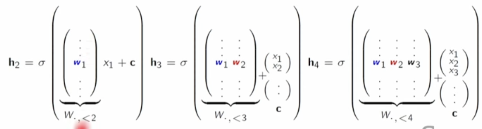
Using a single hidden layer with dimension \(d\), the number of parameters is \(O(nd)\).
60.1.3 RNADE
This is to model continuous data without discretizing it. This is done by making \(\hat{x}_i\) parameterize a continuous distribution. One example is using a mixture of \(K\) Gaussians.
60.2 Autoencoders vs Autoregressive Models
A vanilla autoencoder isn’t a generative model because it can’t be used to generate new data points.
An autoencoder doesn’t enforce an ordering on the input variables. If it does, it becomes an autoregressive model. To make the autoencoder a generative model, you have to make it correspond to a valid Bayesian Network (DAG).
Using masks (a masked autoencoder), you can enforce the DAG structure.
60.3 Recurrent Neural Networks (RNNs)
RNNs keep a summary of the previously seen history (the past random variables) and keep updating it as new information becomes available. The number of parameters is constant in terms of \(n\).
They are very slow in training because the calculation is sequential. Another issue is using only a single vector to summarize all the history. This eases computation but is a huge assumption.
60.4 Attention-Based Models
Attention-based models can access the hidden vectors for all the previous tokens when predicting a new one. This is in contrast to the single vector used in RNNs.
This is done by comparing the set of query vectors with the new key vector. These values are then merged together based on some method that decides which query vectors to focus on more.
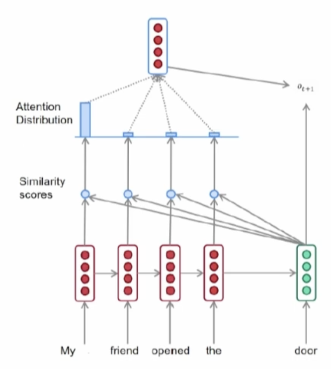
The merged vector is then used to predict the next token.
60.5 CNNs
To use them in autoregressive models, you have to make sure the convolutions respect your selected ordering and the model doesn’t peek into upcoming variables (pixels in the case of working on images). This can be done using masked convolutions.
60.6 Disadvantages of Autoregressive Models
They are very hard to use for representation learning and unsupervised learning.