Variational Autoencoders (VAE)
Latent Variable Models
Latent variables \(\mathbf{z}\) are hidden variables used to capture sources of variability in the data that aren’t explicitly stated (e.g., gender, eye color, pose, hair color in human face images). These variables are initialized randomly and trained through unsupervised learning. You may then build a model that reasons conditioned on the latent variables. This is usually easier because latent variables usually have a smaller dimension. That is \(p(\mathbf{x} | \mathbf{z})\) is easier to model than \(p(\mathbf{x})\). These variables usually correspond to high-level features.
Neural networks can be used to model the conditionals (deep latent variable models. Examples:
\[ \mathbf{z} \sim \mathcal{N}(0, I) \]
\[ p(\mathbf{x} | \mathbf{z}) = \mathcal{N}(\mu_\theta(\mathbf{z}), \Sigma_\theta(\mathbf{z})) \]
where \(\mu_\theta(\mathbf{z})\) and \(\Sigma_\theta(\mathbf{z})\) are neural networks.
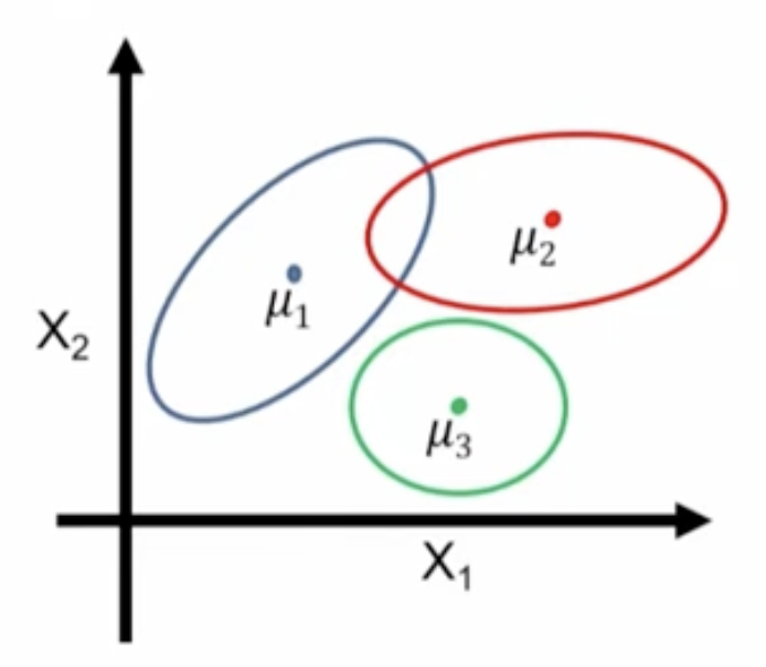
Mixture of Gaussians
This is a Bayes net \(\mathbf{z} \rightarrow \mathbf{x}\) where
\[ \mathbf{z} \sim \text{Categorical}(1, ..., K) \]
\[ p(\mathbf{x} | \mathbf{z} = k) = \mathcal{N}(\mu_k, \sigma_k) \]
Mixture Models
Using latent variables allows us to formulate \(p(x)\) as a mixture of simpler models, creating a complex model from simpler ones. This is because
\[ p(\mathbf{x}) = \sum_z p(\mathbf{x}, \mathbf{z}) = \sum_z p(\mathbf{z})p(\mathbf{x} | \mathbf{z}) \]
Variational Autoencoder
A mixture of an infinite number of Gaussians.
\[ \mathbf{z} \sim \mathcal{N}(0, I) \]
\[ p(\mathbf{x} | \mathbf{z}) = \mathcal{N}(\mu_\theta(\mathbf{z}), \Sigma_\theta(\mathbf{z})) \]
where \(\mu_\theta(\mathbf{z})\) and \(\Sigma_\theta(\mathbf{z})\) are neural networks.
There is an infinite number of Gaussians because \(\mathbf{z}\) is now continuous.
Once again, \(p(\mathbf{x} | \mathbf{z})\) is simple but \(p(\mathbf{x})\), the mixture, is complex.
Calculating the probability of observing a certain training data point, \(\bar{x}\), because it involves calculating an integral
\[ \int_{\mathbf{z}} p(\mathbf{X} = \mathbf{\bar{x}}, \mathbf{Z} = \mathbf{z}, \theta) \,d\mathbf{z} \]
In our setting, we have a dataset \(\mathcal{D}\) where for each datapoint \(\mathbf{X}\) are observed, but the variables \(\mathbf{Z}\) are never observed.
To train the model with maximum likelihood learning, we need to find \(\theta\) that maximizes
\[ \sum_{\mathbf{x} \in \mathcal{D}} \log p(\mathbf{x}, \theta) = \sum_{\mathbf{x} \in \mathcal{D}} \log \sum_{\mathbf{z}} p(\mathbf{x}, \mathbf{z}, \theta) \]
Evaluating \(\sum_{\mathbf{z}} p(\mathbf{x}, \mathbf{z}, \theta)\) is intractable. For example, having 30 binary latent variables will involve the sum of \(2^{30}\) terms. For continuous, the computation is also hard. The gradients with respect to \(\theta\) are also hard to compute.
You could use Monte Carlo to approximate the hard-to-compute sum.
This is because
\[ p_{\theta}(x) = \sum_{\text{All values of }\mathbf{z}} p_{\theta}(\mathbf{x}, \mathbf{z}) = |\mathcal{Z}|\sum_{\mathbf{z} \in \mathcal{Z}} \frac{1}{|\mathcal{Z}|} p_{\theta}(\mathbf{x}, \mathbf{z}) = |\mathcal{Z}| \mathbb{E}_{\mathbf{z} \sim Uniform(\mathcal{Z})} [p_{\theta}(\mathbf{x}, \mathbf{z})] \]
Monte Carlo approximates the expected value through sampling \(k\) values for \(\mathbf{z}\) uniformly at random and approximating using
\[ |\mathcal{Z}| \frac{1}{k} \sum_{j=1} ^ {k} p_{\theta}(\mathbf{x}, \mathbf{z}^{(j)}) \]
The problem here is that uniformly sampling \(\mathbf{z}\) won’t work in the real world, and we need a smarter way.
A better way is to use importance sampling.
\[ p_{\theta}(x) = \sum_{\text{All values of }\mathbf{z}} p_{\theta}(\mathbf{x}, \mathbf{z}) = \sum_{\mathbf{z} \in \mathcal{Z}} \frac{q(\mathbf{z})}{q(\mathbf{z})} p_{\theta}(\mathbf{x}, \mathbf{z}) = \mathbb{E}_{\mathbf{z} \sim q(\mathbf{z})} \frac{p_{\theta}(\mathbf{x}, \mathbf{z})}{q(\mathbf{z})} \]
and once again apply Monte Carlo, but this time sample from \(q(\mathbf{z})\).
Now we also need to train \(q(\mathbf{z})\) which will also be a neural network. We need to minimize \(\log p_{\theta}(\mathbf{x})\) . We can directly minimize this value, but we can minimize a lower bound for it
\[ \log p_{\theta}(\mathbf{x}) = \log \sum_{\mathbf{z}} q(\mathbf{z}) \frac{p_{\theta}(\mathbf{x}, \mathbf{z})}{q(\mathbf{z})} \ge \sum_{\mathbf{z}} q(\mathbf{z}) \log [\frac{p_{\theta}(\mathbf{x}, \mathbf{z})}{q(\mathbf{z})}] = \sum_{\mathbf{z}} q(\mathbf{z}) \log p_{\theta}(\mathbf{x}, \mathbf{z}) - \sum_{\mathbf{z}} q(\mathbf{z}) \log q(\mathbf{z}) = \sum_{\mathbf{z}} q(\mathbf{z}) \log p_{\theta}(\mathbf{x}, \mathbf{z}) + H(q) \]
where the inequality follows from Jensen’s inequality and the fact that the \(\log\) function is concave and \(H(q)\) is the entropy of \(q\). This inequality holds for any \(q\) with it being an equality if \(q = p_{\theta}(\mathbf{z} | \mathbf{x})\). That is the optimal choice of \(q\) is \(p_{\theta}(\mathbf{z} | \mathbf{x})\). We should try to choose \(q\) as close as possible to \(p_{\theta}(\mathbf{z} | \mathbf{x})\).
In practice, we will train together \(q(\mathbf{z})\) (an encoder) and \(p(\mathbf{x} | \mathbf{z})\) (a decoder) to minimize the ELBO.