Chapter 2: Parallel Hardware and Parallel Software
Some Background and Review
The Von Neumann Architecture
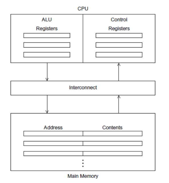
Main Memory
A collection of locations, each of which is capable of storing both instructions and data. Each location has a unique address used to access its content.
Central Processing Unit (CPU)
Contains two components
- Control Unit: Responsible for deciding which instructions should be executed
- Arithmetic and Logic Unit (ALU): Executes the actual instructions
Other Terms
Register: Very fast storage. Part of the CPU.
Program Counter (PC): A register. Stores the address of the next instruction to be executed.
Bus: Connects the CPU and memory
In the Von Neumann architecture, the bottleneck is the connection between the CPU and the memory.
Processes and Threads
A process is an instance of a program that is being executed. It contains
The executable program
A block of memory
Description of resources given by the OS to the process
Security Information
Information about process state
Multitasking gives the illusion that a single processor (with a single core) is running multiple programs simultaneously. It does so by giving each process a chunk of time to run (time slice). After time ends, the process blocks (waits for its next turn.
Threads are contained within processes. A programmer can divide the program into different, sort of independent threads. This is done so that while one thread awaits a resource, other threads can work and perform some tasks. Starting a thread is called forking, while terminating one is called joining.
Modifications to the Von Neumann model
Caching
Caches are built to be accessed faster than the main memory. A CPU cache is usually located on the same chip and accessing it is much faster than accessing ordinary memory.
Usually, designers exploit the principle of locality. Locality is the principle that an access of one memory location is followed by an access of a nearby location. A program typically follows one access by accessing a nearby location (spatial locality) in the near future (temporal locality).
Typically, caches are built on multiple levels (small and fast cache layers followed by larger but slower ones).
When the CPU visits the cache to access a value and finds it, it is called a cache hit. A cache miss is if the CPU doesn’t find the data in the cache.
When a CPU writes data to cache, the value may be inconsistent with memory. There are two ways to handle this:
Write Through Cache: Updates the memory once the cache is updates
Write Back: Marks the data in the cache as dirty. When the value in the cache is being replaced, the dirty line is updated in the memory.
Cache mapping is the issue of mapping memory locations with cache locations. 3 important mappings are:
Full Associative: a new line can be placed anywhere in the cache
Direct Mapped: Each cache line has a unique location in the cache. That is, each memory location can go to only one cache location.
\(n\)-way set associative: Each cache line can be a place for one of \(n\) different cache locations.
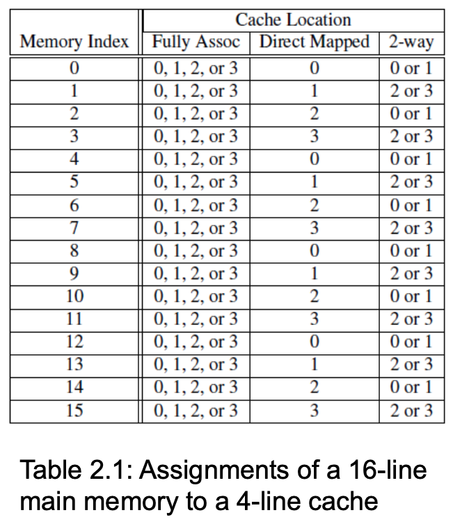
Figure fig-cache-mapping displays the difference between the 3 cache mapping techniques.
Virtual Memory
If you run multiple programs simultaneously, the memory won’t be able to store them all. Virtual paging acts like a cache for secondary storage.
The program is divided into pages (blocks of data and instructions), with some pages stored in memory while others in storage. Pages in secondary storage are swapped when they are needed.
When a program is compiled, its pages are assigned virtual page numbers. When the program is run, a page table is created to map virtual addresses into physical addresses. Since using a page table can increase overall run-time, translation lookaside buffer (TLB) is used to cache values from the page table.
Instruction Level Parallelism (ILP)
Instruction-level parallelism attempts to improve performance by having multiple processor components (or functional units) simultaneously execute instructions.
Pipelining
Functional units are arranged in stages, with these stages running together at the same time.
Multiple Issue
Multiple issue processors replicate functional units (for example, have multiple adders) and try to simultaneously execute different instructions in a program. There are two types:
Static Multiple Issue: Functional units are scheduled at compile time
Dynamic Multiple Issue: Functional units are scheduled at run-time. Also called superscalar execution.
To use multiple issue, the compiler must find instructions that can be executed simultaneously. Speculation is when the processor makes a guess about an instruction and executes it based on the guess.
Hardware Multithreading
Hardware multithreading provides a means for systems to continue doing useful work when the task being currently executed has stalled. There are two types:
Fine-grained: the processor switches between threads after each instruction, skipping threads that are stalled.
Coarse-grained: only switches threads that are stalled waiting for a time-consuming operation to complete
Parallel Hardware
Flynn’s taxonomy divides data processors into 4 types:
SISD: Single Instruction Single Data (That’s classic Von Neumann)
SIMD: Single Instruction Multiple Data
MISD: Multiple Instruction Single Data
MIMD: Multiple Instruction Multiple Data
SIMD
In SIMD, parallelism is achieved through dividing data on processors (data parallelism).
Vector processors are one type of SIMD. They operate on vectors of data.
The current generation of GPUs isn’t pure SIMD, but it uses SIMD parallelism. GPUs run a pipeline of shader functions. These shader functions are parallel, which allows SIMD.
MIMD
MIMD typically consists of a collection of fully independent processing units or cores, each of which has its own control unit and its own ALU. There are two principal types of MIMD systems: shared-memory systems and distributed-memory systems.
Shared Memory Systems
A collection of independent processes is connected to a shared memory. Each process can access all memory locations, and they usually communicate explicitly using shared data structures. Multicore processors are an example of shared memory systems.
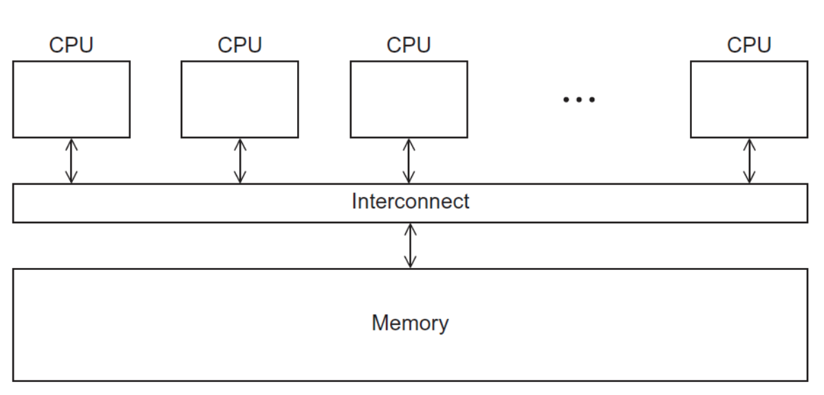
Shared memory systems can be further divided into two types. In Uniform Memory Access systems (UMA), the time to access all the memory locations will be the same for all the cores. In Non-Uniform Memory Access (NUMA), some cores might be directly connected to some memory locations (fast access) and indirectly connected (slow access) to others.
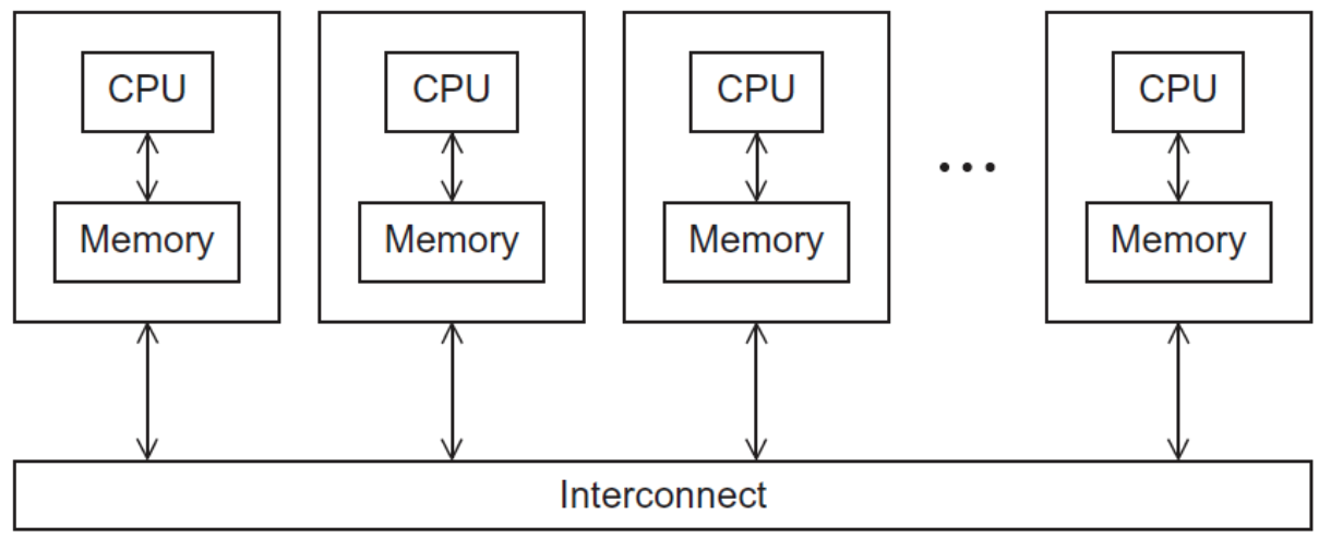
Distributed Memory Systems
The most widely available distributed-memory systems are called clusters. They are composed of a collection of commodity systems—for example, PCs—connected by a commodity interconnection network—for example, Ethernet.
Interconnection Networks
The interconnection network choice affects the performance of both shared and distributed memory systems.
Distributed Memory Interconnects
Distributed memory interconnects can be divided into two types
Direct Interconnects: Each switch is directly connected to a memory processor pair, and the switches are connected to each other.
Indirect Interconnects: Switches may not be directly connected to a processor.
Before we get into specific interconnects of both types, let’s talk about some properties to characterize networks.
Interconnect Networks Characteristics
Bisection Width is a measure of the number of simultaneous communications allowed by the network. It can be calculated in two ways. To understand this measure, imagine that the parallel system is divided into two halves, and each half contains half of the processors or nodes. How many simultaneous communications can take place “across the divide” between the halves?
An alternative way of computing the bisection width is to remove the minimum number of links needed to split the set of nodes into two equal halves. The number of links removed is the bisection width.
The Bandwidth of a link is the rate at which it can transmit data. It’s usually given in megabits or megabytes per second.
Bisection bandwidth is often used as a measure of network quality. Instead of counting the number of links joining the halves as in bisection width, it sums the bandwidth of the links.
Whenever data is being transmitted (on a network, cache-memory, cache-processor), we are interested in the speed of the process. Two measures are
Latency: the time that elapses between the source’s beginning to transmit the data and the destination’s starting to receive the first byte
Bandwidth: The rate at which the destination receives data after it has started to receive the first byte
\[ \text{Message Transmission Time} = l + \frac{n}{b} \]
where \(l\) is the latency in seconds, \(n\) is the message size in bytes, and \(b\) is the bandwidth in bytes per second.
Direct Interconnects
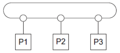
Ring
- Bisection Width: 2
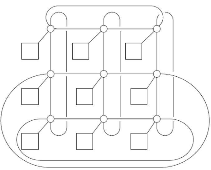
Toroidal Mesh
Description: 2D grid of rings
Bisection Width: \(2\sqrt{p}\)
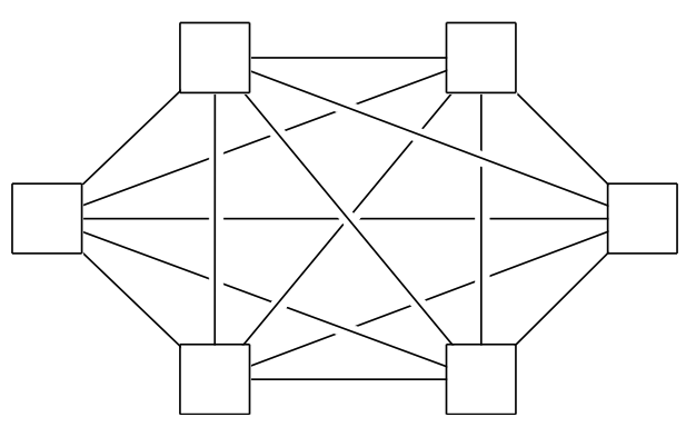
Fully Connected Network
Description: Each switch is directly connected to every other switch.
Optimal Solution
Bisection Width: \(p^2/4\)
Impractical in the real world due to cost (Required number of links \(p^2/2 + p/2\)
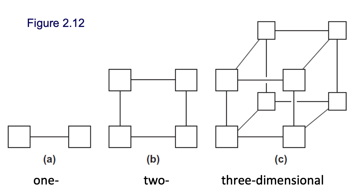
Hypercube
Description: A highly connected direct interconnect that’s built inductively and has been used in the real world
Bisection Width: \(p/2\)
Indirect Interconnects
Their general shape is a group of processor-memory pairs with directed links entering a switching network and each processor is connected with one link coming out from the switch. Check Figure fig-indirect-network.
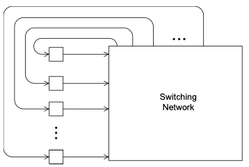
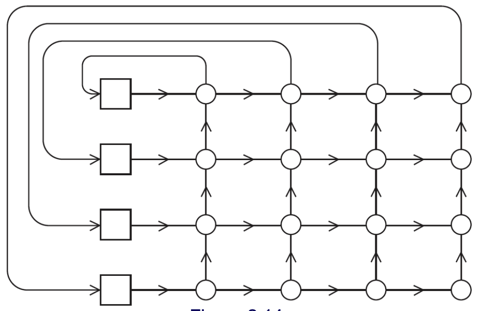
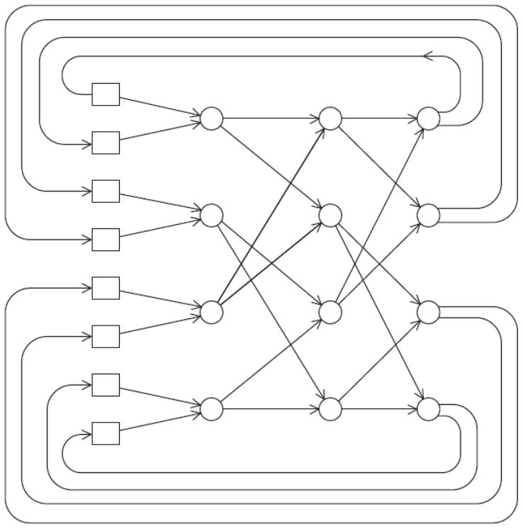
Two examples are the Omega Network and Crossbar. As long as two processors don’t attempt to communicate with the same processor, all the processors can simultaneously communicate with another processor.
TODO: Cache Coherence
Parallel Software
In shared memory (like multicore processors), we start a single process and form threads. In distributed memory, start multiple processes.
A Single Program Multiple Data (SPMD) program contains a single executable that behave differently on each processor using branching.
In shared memory systems, there are two ways of threading. In Dynamic Threading, the master thread waits for work, dynamically creating new threads as needed and removing them when they finish. In Static Threading, a pool of threads is created in the beginning and is terminated only in the cleanup.
In a distributed memory system, only process 0 can access stdin, but all processes can access stdout. Still, it is suggested that only one process uses stdout for determinism. Moreovoer, only a single process/thread can access any single file (only private files; no shared files).
Performance
Speedup
\[ \text{Speedup} = \frac{T_\text{Serial}}{T_\text{Parallel}} \]
The biggest possible speedup value is \(p\) where \(p\) is the number of processors. This is called linear speedup.
Speedup tends to increase as \(p\) increases until it plateaus. As the data size increases, speedup tends to increase as there is usually less overhead.
Efficency
\[ \text{Efficency} = \frac{\text{Speedup}}{p} \]
The highest possible value is 1. Occurs only if there is linear speedup.
Efficency tends to decrease as \(p\) increases. As the data size increases, efficiency tends to increase (approach 1).
Amdahl’s Law
Amdahl’s law provides an upper bound on the speedup that can be obtained by a parallel program.
Let \(f\) be the maximum serializable fraction of the system. Then the minimum \(T_\text{Parallel}\) is
\[ T_\text{Parallel} = \frac{f \times T_\text{Serial}}{p} + (1-f) \times T_\text{Serial} \]
Making the maximum achievable speedup
\[ \text{Speedup} = \frac{1}{\frac{f}{p} + 1 - f} \]
Scalability
In general, a problem is scalable if it can handle ever-increasing problem sizes.
If we increase the number of processes/threads and keep the efficiency fixed without increasing problem size, the problem is strongly scalable.
If we keep the efficiency fixed by increasing the problem size at the same rate as we increase the number of processes/threads, the problem is weakly scalable.